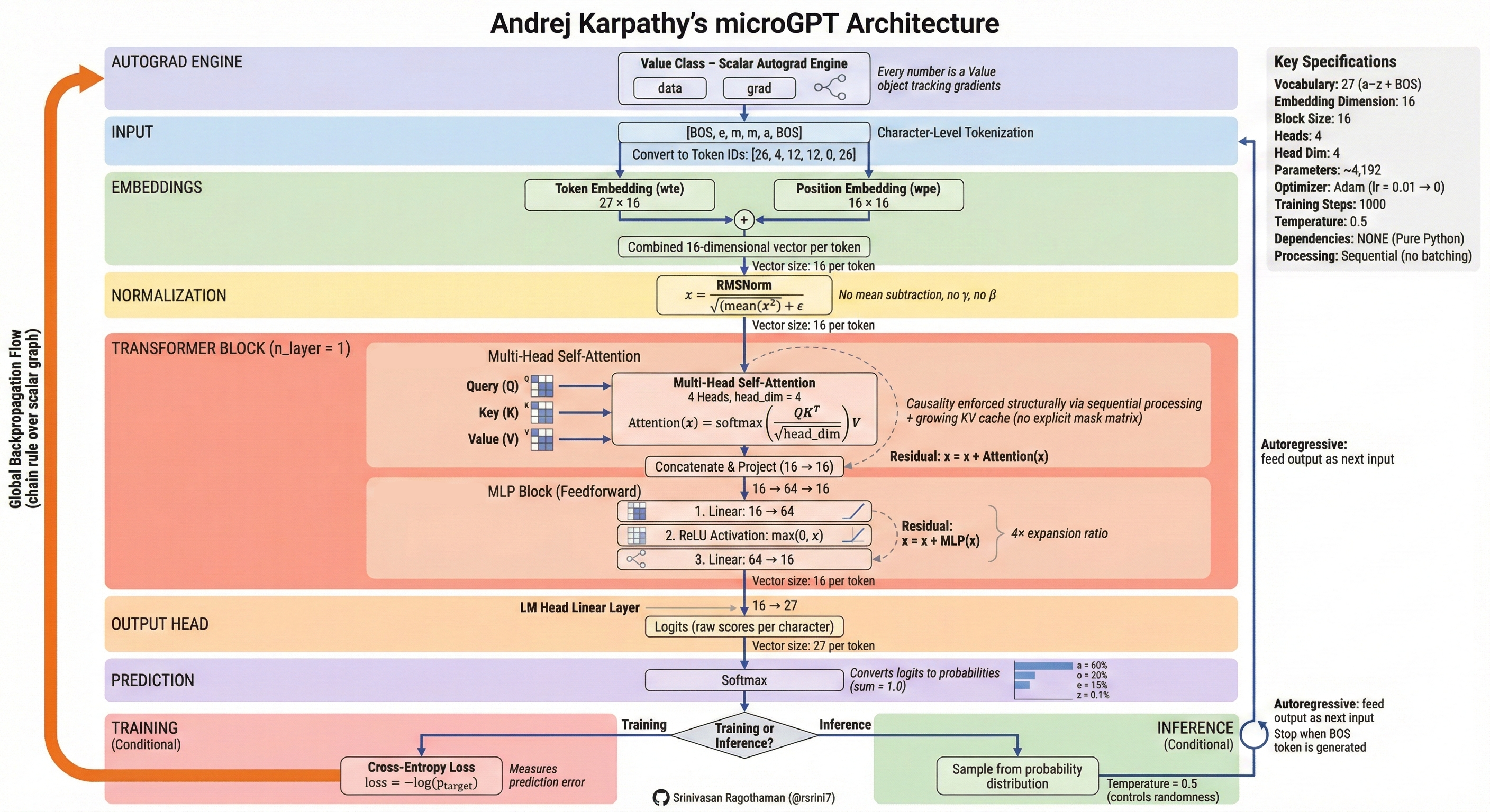
microGPT Architecture — Complete Guide

A comprehensive walkthrough of Andrej Karpathy's microGPT: the "most atomic" GPT implementation using pure Python and math only — no PyTorch, no NumPy, no GPU.

High-Level Overview

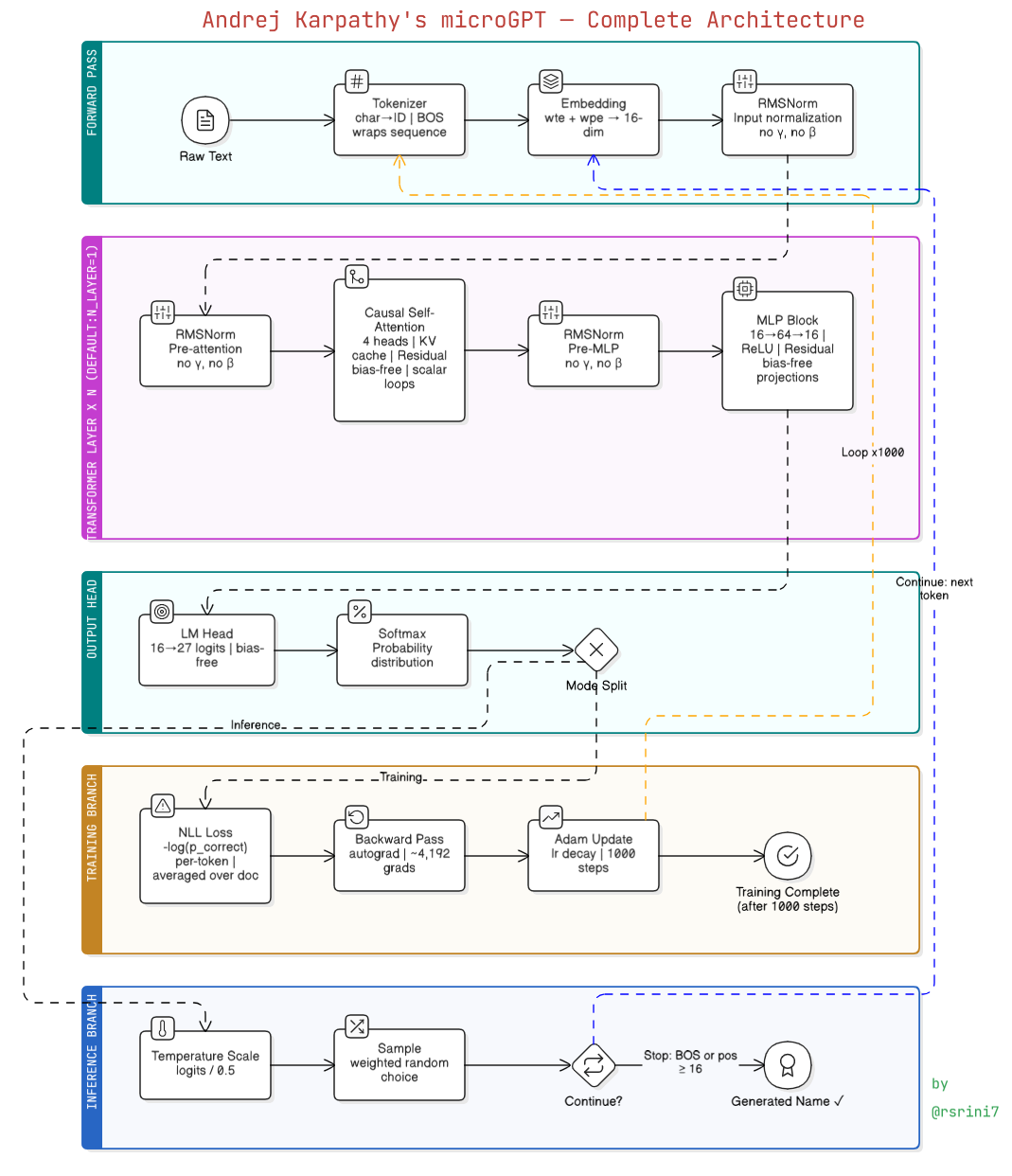
flowchart TD
    A["📄 Raw Text<br/> (names.txt / shakespeare)"] --> B["🔤 Tokenizer<br/> Char → ID"]
    B --> C["📦 Embeddings<br/> Token + Position"]
    C --> D1["📐 RMSNorm ①<br/> After Embedding"]
    D1 --> D2["📐 RMSNorm ②<br/> Before Attention"]
    D2 --> E["🔍 Causal Self-Attention<br/> 4 Heads, KV Cache"]
    E --> D3["📐 RMSNorm ③<br/> Before MLP"]
    D3 --> F["🧠 MLP Block<br/> 16 → 64 → 16"]
    F --> G["📊 LM Head<br/> Logits (27 scores)"]
    G --> H["📈 Softmax<br/> Probabilities"]
    H -->|Training| I["⚖️ Loss + Backprop<br/> → Adam Update"]
    H -->|Inference| J["🎲 Sample<br/> Next Character"]
    J -->|Loop until BOS| J

1. Data Loading and Preprocessing

The script begins by ensuring input.txt exists, defaulting to a dataset of names. Each line (name) is treated as an individual document and shuffled so the model learns character patterns — not a fixed ordering.

if not os.path.exists('input.txt'):
    # downloads names.txt ...
docs = [l.strip() for l in open('input.txt').read().strip().split('\n') if l.strip()]
random.shuffle(docs)

2. The Tokenizer — Text to Numbers

This is not a fancy library tokenizer. It finds every unique character in the text and uses that as the vocabulary.

uchars = sorted(set(''.join(docs)))
BOS = len(uchars)   # Beginning of Sequence token (also acts as End-of-Sequence)
vocab_size = len(uchars) + 1

A special BOS token is added — it serves as both the start signal during generation and the stop signal when it's sampled as output.

Example:

"emma" → [BOS, e, m, m, a, BOS] → [26, 4, 12, 12, 0, 26]

flowchart LR
    T["'emma'"] --> C1["e → 4"]
    T --> C2["m → 12"]
    T --> C3["m → 12"]
    T --> C4["a → 0"]
    BOS1["BOS → 26"] --> E
    C1 --> E["[26, 4, 12, 12, 0, 26]"]
    C2 --> E
    C3 --> E
    C4 --> E
    BOS2["BOS → 26"] --> E

3. Embeddings — Numbers to Meaningful Vectors

Each token ID gets two 16-dimensional vectors that are added together to form one input vector:

Embedding	Weight Matrix	Encodes
Token Embedding (wte)	`state_dict['wte'][token_id]`	What this character is
Position Embedding (wpe)	`state_dict['wpe'][pos_id]`	Where this character sits in the sequence

flowchart LR
    TID["token_id = 4 (e)"] --> WTE["wte lookup<br/> → 16-dim vector"]
    PID["pos_id = 1"] --> WPE["wpe lookup<br/> → 16-dim vector"]
    WTE --> ADD["➕ Element-wise Add"]
    WPE --> ADD
    ADD --> X["x: input vector<br/> [16 floats]"]

wte — Token Embedding Table

It encodes "What" — the identity of the character itself. Each character in the vocabulary gets its own unique 16-dimensional vector. So "e" always starts with the same base vector regardless of where it appears in a word. It's looked up by token_id.

tok_emb = state_dict['wte'][token_id]  # "who is this character?"

wpe — Position Embedding Table

It encodes "Where" — the position of the character in the sequence. Position 0 has its own 16-dim vector, position 1 has another, and so on up to block_size. This tells the model where in the sequence the current character sits.

pos_emb = state_dict['wpe'][pos_id]   # "where in the sequence?"

Together:

x = [t + p for t, p in zip(tok_emb, pos_emb)]

They are element-wise added to produce one combined 16-dim vector that carries both pieces of information — identity + position — before being passed into the Transformer. Without wpe, the model would treat "e" at position 1 the same as "e" at position 5, losing all sense of word structure.

4. RMSNorm — Stabilize the Numbers

microGPT uses a pre-norm Transformer design: RMSNorm is applied before each sublayer (attention and MLP) inside each Transformer block, plus once at input after the combined embedding. This keeps values in a stable range and prevents exploding/vanishing gradients.

x = rmsnorm(x)            # at input — after embedding, before the layer block
# inside each layer:
x = rmsnorm(x)            # before attention sublayer
x = rmsnorm(x)            # before MLP sublayer

Formula: x / sqrt(mean(x²) + ε)

Important: This RMSNorm has no learnable parameters — no scale (γ) or shift (β). Unlike LayerNorm, it is purely a normalization operation with nothing added to state_dict.

5. The Autograd Engine — `Value` Class

Value is the minimal building block that replaces PyTorch's entire autograd system. Every scalar number in the model — both weights and intermediate activations — is wrapped in a Value object. Each Value stores three things: its scalar data, its gradient (.grad), and links to its parent nodes (children and local_grads) so the computation graph can be traversed.

class Value:
    def __init__(self, data, children=(), local_grads=()):
        self.data = data       # the scalar value
        self.grad = 0          # gradient accumulates here during backward()
        self._children = children       # parent nodes in the graph
        self._local_grads = local_grads # local derivative w.r.t. each parent
    def backward(self):
        # reverse topological sort + chain rule

flowchart LR
    FWD["Forward Pass<br/> Every math op on Values<br/> builds the graph"] --> GRAPH["🕸️ Computation Graph<br/> (Values linked via children/local_grads)"]
    GRAPH --> BWD["loss.backward()<br/> Walk in reverse<br/> topological order"]
    BWD --> GRAD["Gradients accumulate<br/> in each node's .grad<br/> (~4,192 total)"]
    GRAD --> ADAM["Adam reads .grad<br/> to update weights"]

Forward pass: every math operation (+, *, log, etc.) records its inputs as children and stores the local derivative as local_grads, building the graph automatically.
Backward pass: loss.backward() performs a reverse topological sort of the entire graph and walks it in reverse, applying the chain rule at each node. The gradient of the loss with respect to each parameter accumulates in .grad.
Adam then reads .grad from every parameter Value to perform the weight update — this is the bridge between autograd and the optimizer.

6. Parameter Initialization

Before the model can run, all learnable weight matrices must be created and stored in a state_dict dictionary. There are four core model size hyperparameters that together determine total model capacity:

Hyperparameter	Value	Controls
`n_embd`	16	Width of every vector representation
`n_head`	4	Number of attention heads
`n_layer`	1	Depth — how many Transformer blocks
`block_size`	10	Maximum sequence length the model trains on at once

block_size deserves special attention. Each document is one line from input.txt. If lines are very short (like names: 3–8 characters), block_size rarely becomes a limiting factor — the whole name fits within it easily. But if lines are long (like Shakespeare passages), block_size controls how much of the line the model can see as context at any one position. A small block_size means the model only ever sees a short window, which is a direct reason it cannot learn long-range patterns — it never has access to context from far back in the sequence. This is explicitly why the Shakespeare experiment produces words and local formatting but lacks real structural memory.

Every matrix is seeded with small random numbers via a helper matrix() function that returns a 2D list of Value objects.

n_embd   = 16   # embedding dimension
n_head   = 4    # attention heads
n_layer  = 1    # transformer layers
block_size = 10 # max sequence length

state_dict = {
    'wte': matrix(vocab_size, n_embd),   # token embedding table
    'wpe': matrix(block_size, n_embd),   # position embedding table
}
for i in range(n_layer):
    state_dict[f'layer{i}.attn_wq'] = matrix(n_embd, n_embd)  # Query projection
    state_dict[f'layer{i}.attn_wk'] = matrix(n_embd, n_embd)  # Key projection
    state_dict[f'layer{i}.attn_wv'] = matrix(n_embd, n_embd)  # Value projection
    state_dict[f'layer{i}.attn_wo'] = matrix(n_embd, n_embd)  # Output projection
    state_dict[f'layer{i}.mlp_fc1'] = matrix(n_embd, n_embd * 4)  # MLP expand
    state_dict[f'layer{i}.mlp_fc2'] = matrix(n_embd * 4, n_embd)  # MLP contract
state_dict['lm_head'] = matrix(n_embd, vocab_size)             # final classifier

flowchart LR
    DIM["Dimensions<br/> n_embd=16, n_head=4"] --> WTE["wte<br/> vocab_size × 16"]
    DIM --> WPE["wpe<br/> block_size × 16"]
    DIM --> ATT["Attention matrices<br/> wq, wk, wv, wo<br/> (each 16 × 16)"]
    DIM --> MLP["MLP matrices<br/> fc1: 16 × 64<br/> fc2: 64 × 16"]
    DIM --> LMH["lm_head<br/> 16 × vocab_size"]
    WTE & WPE & ATT & MLP & LMH --> SD["state_dict<br/> ~4,192 total params"]

All matrices are bias-free. Every linear projection in this model computes only Wx — there is no + b term anywhere. The params list flattens all Value objects from state_dict for the optimizer to iterate over.

7. Model Architecture — `gpt()` Function

The gpt function is the Transformer. It processes one token at a time — there is no batching, no batch dimension, no parallel sequence processing. This single-token-at-a-time design is exactly why causality is structural: the KV cache simply hasn't seen future tokens yet when the current one is processed.

All linear projections (Q, K, V, attn_wo, mlp_fc1, mlp_fc2, lm_head) are bias-free — the linear() function computes only Wx, never Wx + b. This matches modern GPT design.

def gpt(token_id, pos_id, keys, values):
    tok_emb = state_dict['wte'][token_id]
    pos_emb = state_dict['wpe'][pos_id]
    x = [t + p for t, p in zip(tok_emb, pos_emb)]
    x = rmsnorm(x)
    # ... Attention and MLP blocks ...

7a. Causal Self-Attention

flowchart TD
    X["Input x [16-dim]"] --> Q["Query (Q)<br/> 'What am I looking for?'"]
    X --> K["Key (K)<br/> 'What info do I have?'"]
    X --> V["Value (V)<br/> 'What do I share?'"]
    Q --> SCORE["Attention Scores<br/> Q·Kᵀ / √(head_dim)"]
    K --> SCORE
    SCORE --> SOFT["Softmax → weights<br/> ⚠️ No mask tensor — KV cache<br/> only holds past positions<br/> (implicit causality)"]
    SOFT --> OUT["Weighted sum of Values"]
    V --> OUT
    OUT --> HEADS["4 Heads concatenated<br/> (each head: 4-dim output)<br/> 4 × 4 = 16-dim total"]
    HEADS --> PROJ["attn_wo: Linear 16 → 16<br/> (output projection)"]
    X --> RES["➕ Residual Connection<br/> x = x + Attention(x)"]
    PROJ --> RES

Key insight on causality: There is no explicit masking matrix. Causality is enforced structurally — at position 5, the KV cache only contains entries from positions 0–4 because they haven't been processed yet.

keys[li].append(k)
values[li].append(v)
# Scores are only computed over the keys seen so far
attn_logits = [sum(q_h[j] * k_h[t][j] for j in range(head_dim))
               for t in range(len(keys[li]))]

Head dimension arithmetic: head_dim = n_embd // n_head = 16 // 4 = 4. Each of the 4 heads independently attends over its own 4-dimensional slice of Q, K, V. Their outputs are concatenated back to 16 dims, then passed through attn_wo (a 16×16 linear projection) before the residual add.

Implementation note: There are no tensor matmul operations. Attention scores are computed via explicit Python loops over scalars: sum(q_h[j] * k_h[t][j] for j in range(head_dim)). Everything is scalar arithmetic on Value objects.

7b. MLP Block

flowchart LR
    X16["x [16-dim]"] --> FC1["Linear: 16 → 64"]
    FC1 --> RELU["ReLU<br/> (negatives → 0)"]
    RELU --> FC2["Linear: 64 → 16"]
    FC2 --> RES["➕ Residual<br/> x = x + MLP(x)"]
    X16 --> RES

The expansion to 64 dimensions gives the model more "room to think" before compressing back.

8. LM Head + Softmax — Scores to Probabilities

flowchart LR
    X16["x [16-dim]"] --> HEAD["Linear projection<br/> 16 → 27 logits"]
    HEAD --> SOFT["Softmax"]
    SOFT --> PROBS["Probabilities<br/> 'a':60%, 'o':20%, 'z':0.1%..."]

The 27 scores (one per character in the vocabulary) are converted to a probability distribution that sums to 100%.

9. Training Loop — Learning from Mistakes

Task: Next Token Prediction. If the model sees "J", it tries to predict "e" for "Jeffrey".

On each training step, one document (one line) is picked from docs. It is tokenized as [BOS] + characters + [BOS]. The number of positions actually trained is:

n = min(block_size, len(doc_tokens) - 1)

This caps training at block_size even if the document is longer, and subtracts 1 because next-token prediction needs a target at t+1 for every input at t. After the forward pass, loss is averaged across all positions in that document, gradients are computed, Adam updates the weights, and gradients are reset to zero before the next document.

losses = []
for pos_id in range(n):
    token_id, target_id = tokens[pos_id], tokens[pos_id + 1]  # current → next
    logits = gpt(token_id, pos_id, keys, values)
    probs = softmax(logits)
    loss_t = -probs[target_id].log()   # .log() is autograd-aware: defined on the Value class
    losses.append(loss_t)
loss = (1 / n) * sum(losses)           # per-token loss averaged across the document slice

flowchart TD
    A["Step 1–7: Forward Pass<br/> → probabilities"] --> L["Step 8: Compute Loss<br/> -log(P(correct char))<br/> High surprise = High loss"]
    L --> B["Step 9: Backpropagation<br/> Autograd traces graph<br/> → 4,192 gradients"]
    B --> O["Step 10: Adam Update<br/> Nudge weights → lower loss"]
    O -->|Next token| A

Loss intuition: If the model predicts the correct next character with low confidence → loss is high. Perfect confidence → loss approaches 0.

10. The Adam Optimizer

lr_t = learning_rate * (1 - step / num_steps)  # linear decay
for i, p in enumerate(params):
    m[i] = beta1 * m[i] + (1 - beta1) * p.grad        # 1st moment (mean)
    v[i] = beta2 * v[i] + (1 - beta2) * p.grad ** 2   # 2nd moment (variance)
    m_hat = m[i] / (1 - beta1 ** (step + 1))           # bias correction
    v_hat = v[i] / (1 - beta2 ** (step + 1))           # bias correction
    p.data -= lr_t * m_hat / (v_hat ** 0.5 + eps_adam) # weight update
    p.grad = 0                                          # zero out gradient

flowchart LR
    G["Gradient p.grad"] --> M["1st Moment Buffer m<br/> (smoothed mean)"]
    G --> V["2nd Moment Buffer v<br/> (smoothed variance)"]
    M --> ADAM["Adam Update<br/> w = w - lr * m̂/√v̂"]
    V --> ADAM
    ADAM --> W["Updated Weight"]

The moment buffers act as memory for training — they smooth out updates so learning doesn't wobble, ensuring convergence.

Learning rate starts at 0.01 and follows linear decay to 0: lr_t = 0.01 × (1 − step/1000). Gradient is zeroed after each update (p.grad = 0) since the Value engine accumulates.

11. Inference — Generating New Names

temperature = 0.5  # controls randomness: low = conservative, high = creative
for pos_id in range(block_size):
    logits = gpt(token_id, pos_id, keys, values)
    probs = softmax([l / temperature for l in logits])  # temperature applied to logits BEFORE softmax
    token_id = random.choices(range(vocab_size), weights=[p.data for p in probs])[0]
    if token_id == BOS:
        break  # Stop if it predicts the end

Note on temperature: dividing logits by a value < 1 sharpens the distribution (more confident), while > 1 flattens it (more random). The source uses temperature = 0.5 by default.

flowchart TD
    START["Start: BOS token"] --> FWD["Forward Pass<br/> → probabilities"]
    FWD --> SAMPLE["Sample next character<br/> (weighted random)"]
    SAMPLE --> CHECK{Is it BOS<br/> or max length?}
    CHECK -->|No| APPEND["Append to sequence"]
    APPEND --> FWD
    CHECK -->|Yes| OUT["Output generated name<br/> e.g. 'emma', 'oliver'"]

Inference is identical to the forward pass during training — but no loss is calculated and no weights are updated. The model "babbles" by feeding its own output back in as the next input (autoregressive generation).

12. Full Training Pipeline — End to End

sequenceDiagram
    participant D as Data
    participant T as Tokenizer
    participant M as Model (gpt)
    participant A as Autograd
    participant O as Adam

    D->>T: Raw characters
    T->>M: Token IDs [BOS, e, m, m, a]
    loop For each position
        M->>M: Embed + Norm + Attention + MLP
        M->>A: Logits → Loss
        A->>A: backward() — compute all gradients
        A->>O: Gradients for 4,192 params
        O->>M: Updated weights
    end
    M-->>D: Repeat for 1,000 steps

13. Model Capacity & Experiments

Experiment	Result
1,000 steps on names	Learns basic name structures — common endings, typical lengths
10,000 steps on names	No clear improvement over 1,000 steps — the task is simple enough that the model saturates quickly
Shakespeare (small model)	Produces basic short words, punctuation, and line breaks, but not real Shakespeare

What the Shakespeare model learns vs misses:

It picks up surface patterns — common short words ("the", "me", "and"), punctuation placement, and line break frequency. What it completely misses is deeper structure: multi-line continuity, rhythmic meter, long-range phrasing, and dramatic coherence. There are three compounding reasons for this:

block_size = 10 — the model never sees more than 10 characters at once, so long-range context is structurally inaccessible
Each line is treated as a separate document — the model has no continuity between lines; every line is an isolated training example, so it never learns cross-line patterns
Tiny capacity — 1 layer, 16-dim embeddings, ~4,192 parameters total is far too small to internalize Shakespeare's vocabulary and structure

Scaling note: Larger GPTs increase n_layer, n_embd, block_size, and vocab_size — but the core algorithm here is identical. Everything else is just efficiency.

14. Key Design Principle

The entire architecture runs on pure Python scalars. Every number is wrapped in a custom Value object that tracks both its value and its gradient, building a computation graph that enables learning via the chain rule.

Characters get personalities (embeddings)
    → talk to each other (attention)
    → think deeply (MLP)
    → predict what comes next (LM head + softmax)
    → learn from mistakes (loss + backprop + Adam)
    → repeat

Based on Andrej Karpathy's microGPT implementation.

rsrini7/microGPT-Architecture-Complete.md

microGPT Architecture — Complete Guide

High-Level Overview

1. Data Loading and Preprocessing

2. The Tokenizer — Text to Numbers

3. Embeddings — Numbers to Meaningful Vectors

4. RMSNorm — Stabilize the Numbers

5. The Autograd Engine — Value Class

6. Parameter Initialization

7. Model Architecture — gpt() Function

7a. Causal Self-Attention

7b. MLP Block

8. LM Head + Softmax — Scores to Probabilities

9. Training Loop — Learning from Mistakes

10. The Adam Optimizer

11. Inference — Generating New Names

12. Full Training Pipeline — End to End

13. Model Capacity & Experiments

14. Key Design Principle

microGPT Architecture — Step-by-Step Flow (Plain English)

Forward Pass (Making Predictions)

Step 1: Tokenizer - Text to Numbers

Step 2: Embeddings - Numbers to Meaningful Vectors

Step 3: RMSNorm - Stabilize the Numbers

Step 4: Attention Layer - Letters Talk to Each Other

Step 5: MLP Block - Deep Thinking

Step 6: LM Head - Turn Thoughts into Character Scores

Step 7: Softmax - Scores to Probabilities

Training Mode - Learning from Mistakes

Step 8: Calculate Loss

Step 9: Backpropagation - Figure Out What Went Wrong

Step 10: Update Parameters with Adam Optimizer

Inference Mode - Generating New Text

Step 11: Autoregressive Generation Loop

Key Principle

🧩 In One Sentence

rsrini7 commented Feb 14, 2026 • edited Loading Uh oh! There was an error while loading. Please reload this page.

Uh oh!

Uh oh!

5. The Autograd Engine — `Value` Class

7. Model Architecture — `gpt()` Function

rsrini7 commented Feb 14, 2026 •

edited

Loading